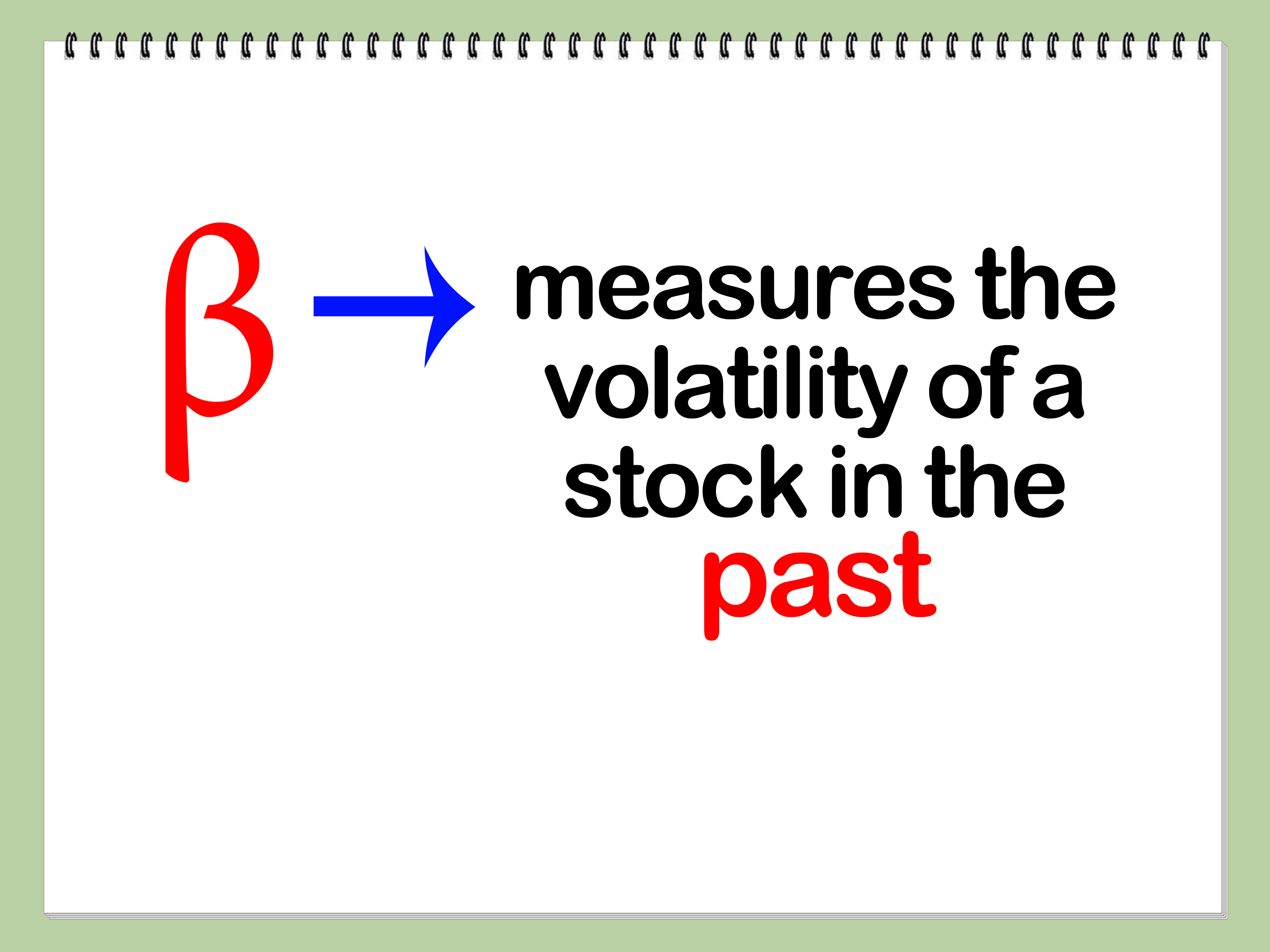
Beta sounds like something that belongs in a science lab, possibly next to a bubbling test tube and a nervous intern. In finance, however, beta is a practical measurement of how strongly a stock, fund, or portfolio has moved in relation to a market benchmark.
Investors use beta to compare market sensitivity, estimate the cost of equity, build portfolios, and evaluate whether an investment tends to behave like a calm commuter train or a roller coaster with questionable safety inspections. A beta of 1.0 suggests that an investment has historically moved with its benchmark. A beta above 1.0 indicates greater sensitivity to market movements, while a beta below 1.0 indicates lower sensitivity.
This guide explains how to calculate beta manually, with regression analysis, in Excel, and for an entire portfolio. It also covers unlevered beta, adjusted beta, common calculation mistakes, and the limitations investors should understand before placing too much faith in one tidy number.
What Is Beta in Finance?
Beta is a statistical measure of an investment’s sensitivity to movements in a selected market benchmark. It focuses on systematic risk, meaning the market-related risk that cannot normally be eliminated simply by owning more securities.
The benchmark is often the S&P 500 for a U.S. stock, but that choice is not mandatory. A technology stock might be compared with the Nasdaq Composite or a technology-sector index. An international fund may need a global or regional benchmark. The calculation only becomes meaningful when the benchmark reasonably represents the market exposure being studied.
Beta is not the same as total volatility. A stock can experience large company-specific price swings while having a modest beta if those movements are weakly related to the broader market. Conversely, a stock may have fewer dramatic surprises but still exhibit a high beta because it consistently magnifies market moves. Beta measures relative market sensitivity, not every possible form of investment risk.
How to Interpret Beta
- Beta of 1.0: The asset has historically moved approximately in line with the benchmark.
- Beta above 1.0: The asset has been more sensitive to benchmark movements.
- Beta between 0 and 1.0: The asset has generally moved in the benchmark’s direction, but less dramatically.
- Beta near 0: The asset has shown little relationship with benchmark returns.
- Negative beta: The asset has tended to move in the opposite direction from the benchmark.
For example, a beta of 1.40 suggests that when the benchmark changes by 1%, the stock has historically changed by roughly 1.40% in the same direction, on average. That does not mean the stock will rise exactly 1.40% whenever the market rises 1%. Markets are not famous for following instructions.
The Formula for Calculating Beta
The standard beta formula is:
Beta = Covariance of stock and market returns / Variance of market returns
Written mathematically:
β = Cov(Ri, Rm) / Var(Rm)
In the formula:
Rirepresents the returns of the stock or other investment.Rmrepresents the returns of the market benchmark.Cov(Ri, Rm)measures how the two return series move together.Var(Rm)measures the dispersion of the benchmark’s returns.
Beta can also be estimated by running a linear regression of the investment’s returns against the benchmark’s returns. The slope of that regression line is beta. In a formal Capital Asset Pricing Model analysis, excess investment returns are commonly regressed against excess market returns.
How to Calculate Beta Step by Step
Step 1: Select an Appropriate Benchmark
Choose a benchmark that matches the investment’s market exposure. The S&P 500 may be suitable for a large U.S. company, but it may be a poor comparison for a small-cap biotechnology stock, a municipal bond fund, or an emerging-market portfolio.
A mismatched benchmark can produce a mathematically correct beta that answers the wrong question. That is rather like calculating how fast a bicycle is by comparing it with a submarine.
Step 2: Choose a Time Period and Return Frequency
Common approaches include three to five years of monthly returns or one to two years of weekly returns. Some financial-data providers calculate beta from 36 or 60 months of historical observations, although methodologies vary among providers.
Daily data supplies more observations but may introduce market noise, thin-trading problems, and timing mismatches. Monthly data is smoother but may react slowly to changes in a company’s business model or financial leverage.
Whatever frequency you choose, use the same dates and frequency for both the asset and the benchmark.
Step 3: Convert Prices into Returns
Beta should be calculated from returns, not from raw stock prices. A basic simple-return formula is:
Return = (Current price - Previous price) / Previous price
Suppose a stock rises from $50 to $52. Its return is:
($52 - $50) / $50 = 0.04, or 4%
For a more complete analysis, use total-return data that accounts for dividends and other distributions. Using adjusted prices helps prevent dividend payments and stock splits from distorting the return series.
Step 4: Calculate Covariance
Covariance indicates whether the stock and benchmark have generally moved together. Positive covariance means they have tended to move in the same direction. Negative covariance means they have tended to move in opposite directions.
Step 5: Calculate Market Variance
Variance measures how widely market returns have fluctuated around their average. Because beta compares the stock’s co-movement with the benchmark against the benchmark’s own variability, market variance appears in the denominator.
Step 6: Divide Covariance by Variance
Once covariance and market variance are known, divide the first number by the second. The result is the investment’s historical beta for the selected data, benchmark, period, and frequency.
A Simple Beta Calculation Example
Assume the following six monthly returns:
| Month | Market Return | Stock Return |
|---|---|---|
| 1 | 2% | 3% |
| 2 | -1% | -2% |
| 3 | 3% | 5% |
| 4 | 0% | 1% |
| 5 | 4% | 6% |
| 6 | -2% | -3% |
Using these observations:
Beta = Covariance of stock and market returns / Variance of market returns
The resulting beta is approximately:
Beta = 1.54
This result suggests that the stock was about 54% more sensitive than the benchmark during the sample period. If the market rose by 1%, the regression relationship would associate that movement with an average stock move of approximately 1.54%, before considering the regression intercept and unexplained company-specific effects.
Six observations are useful for demonstrating the math, but they are far too few for a dependable investment conclusion. A practical estimate should use a longer, consistent return history.
How to Calculate Beta in Excel
Excel makes beta calculation considerably easier. It also reduces the likelihood of spending an afternoon arguing with a calculator.
Assume:
- Column A contains dates.
- Column B contains stock prices.
- Column C contains benchmark prices.
- Column D contains stock returns.
- Column E contains benchmark returns.
Calculate Returns in Excel
In cell D3, enter:
=(B3/B2)-1
In cell E3, enter:
=(C3/C2)-1
Copy both formulas down through the complete data set.
Method 1: Use the SLOPE Function
The quickest Excel beta formula is:
=SLOPE(D3:D62,E3:E62)
The stock-return range comes first because it is the dependent variable. The benchmark-return range comes second because it is the independent variable.
Excel’s SLOPE function returns the slope of the linear regression line, which is the beta estimate.
Method 2: Use Covariance and Variance
You can also calculate beta directly:
=COVARIANCE.S(D3:D62,E3:E62)/VAR.S(E3:E62)
Alternatively, you may use the population versions:
=COVARIANCE.P(D3:D62,E3:E62)/VAR.P(E3:E62)
Use matching conventions. Do not divide sample covariance by population variance or mix the two approaches. Microsoft defines COVARIANCE.P as the population covariance function and VAR.P as the population variance function.
Method 3: Use Excel’s Regression Tool
Enable the Analysis ToolPak, select Data, choose Data Analysis, and select Regression. Use stock returns as the Y range and benchmark returns as the X range.
The coefficient beside the benchmark variable is beta. The regression output also provides useful supporting statistics:
- Intercept: The estimated return when benchmark return is zero.
- R-squared: The percentage of variation in stock returns explained by benchmark returns.
- Standard error: An indication of estimation uncertainty.
- t-statistic and p-value: Measures used to evaluate the statistical significance of the estimated relationship.
A beta number becomes more informative when viewed with R-squared. A beta of 1.50 with a very low R-squared may not describe the stock nearly as well as a beta of 1.10 with a strong benchmark relationship. Microsoft describes R-squared as the proportion of variation in the dependent data attributable to variation in the independent data.
How to Calculate Portfolio Beta
A portfolio’s beta can be estimated as the weighted average of the individual holdings’ betas:
Portfolio beta = Σ(Investment weight × Investment beta)
Suppose a portfolio contains:
- 40% in Stock A, with a beta of 1.40
- 35% in Stock B, with a beta of 0.90
- 25% in cash, with an assumed beta of 0
The calculation is:
(0.40 × 1.40) + (0.35 × 0.90) + (0.25 × 0) = 0.875
The portfolio beta is approximately 0.88. It has historically been less sensitive to market movements than a portfolio with a beta of 1.0. The weighted-average approach is commonly used to estimate portfolio beta when individual asset betas and portfolio weights are available.
Levered Beta and Unlevered Beta
The beta commonly displayed on financial websites is usually an equity beta, also called levered beta. It reflects both the operating risk of the business and the financial risk created by debt.
Analysts often remove the effect of debt when comparing companies with different capital structures.
Unlevered Beta Formula
Unlevered beta = Levered beta / [1 + (1 - Tax rate) × (Debt / Equity)]
Relevered Beta Formula
Relevered beta = Unlevered beta × [1 + (1 - Tax rate) × (Debt / Equity)]
Suppose a comparable company has a levered beta of 1.30, a debt-to-equity ratio of 0.50, and a 25% tax rate:
Unlevered beta = 1.30 / [1 + (1 - 0.25) × 0.50] = 0.95, approximately
If the company being valued has a target debt-to-equity ratio of 0.30:
Relevered beta = 0.95 × [1 + (1 - 0.25) × 0.30] = 1.16, approximately
This bottom-up approach is particularly useful when valuing private companies, newly listed businesses, or public companies whose historical beta may be unreliable. NYU valuation materials describe the same process of unlevering comparable-company betas and relevering them for a target capital structure.
How Beta Is Used in CAPM
Beta is a central input in the Capital Asset Pricing Model:
Expected return = Risk-free rate + Beta × (Expected market return - Risk-free rate)
Assume:
- Risk-free rate: 4%
- Expected market return: 10%
- Stock beta: 1.20
The expected return is:
4% + 1.20 × (10% - 4%) = 11.2%
Businesses use this result as an estimate of the cost of equity in valuation and capital-budgeting models. CAPM links expected return to systematic market risk, although real-world returns can also be influenced by company size, valuation, profitability, momentum, interest rates, and many other factors.
Common Mistakes When Calculating Beta
Using Prices Instead of Returns
Regressing one price series against another can create a misleading relationship because both may trend upward over time. Calculate percentage or logarithmic returns first.
Choosing the Wrong Benchmark
Beta is always relative to something. Changing the benchmark can change the result, sometimes substantially.
Mixing Daily and Monthly Data
The stock and benchmark observations must cover matching dates and intervals. A monthly stock return should not be paired with a weekly index return merely because both numbers were conveniently nearby.
Ignoring Dividends and Stock Splits
Unadjusted closing prices may produce false returns around splits and may understate performance by excluding distributions.
Using Too Few Observations
A beta based on a handful of months can be dominated by one unusual earnings announcement, acquisition, regulatory event, or market panic.
Treating Beta as a Forecasting Machine
Beta describes an estimated historical relationship. It does not guarantee that the relationship will continue, and it does not predict whether the market itself will rise or fall.
Practical Experience and Lessons from Real-World Beta Calculations
In practical financial modeling, the arithmetic is usually the easy part. Entering =SLOPE() takes seconds. Choosing defensible data can take considerably longer. Analysts often discover that two reputable financial websites report different betas for the same company. This does not necessarily mean one website misplaced its calculator. The providers may use different benchmarks, return frequencies, lookback periods, price adjustments, or regression conventions.
A useful first lesson is to record the methodology beside every beta estimate. A number such as 1.27 is incomplete without context. A more informative description would be “five-year monthly beta against the S&P 500 using adjusted total-return data.” That extra sentence can prevent confusion when another analyst calculates 1.11 from two years of weekly observations.
Another recurring lesson is that beta can change when the company changes. A mature software company may acquire a speculative business, borrow heavily, sell a stable division, or become dependent on one volatile product. A five-year beta then blends the company’s old personality with its new one. Using a shorter period may capture current conditions more quickly, but it also produces a noisier estimate. There is no universally perfect window; the choice should match the purpose of the analysis.
Data cleaning also matters more than beginners expect. Missing dates, duplicate rows, dividend payments, stock splits, and differences in market holidays can quietly damage a return series. Before running the regression, analysts should sort observations by date, confirm that stock and benchmark dates match, and investigate unusually large returns. An extreme value may represent a genuine market event, but it may also be a bad price observation wearing a very convincing disguise.
For valuation work, relying on one company’s regression beta is often less reliable than using comparable businesses. A company with a short trading history may produce an unstable beta. A thinly traded stock can appear less sensitive simply because its price does not update frequently. In these cases, analysts commonly collect betas from several comparable companies, remove the effect of each company’s debt, calculate an industry average or median, and then apply the target company’s intended financial leverage.
It is also useful to test several scenarios. Calculate beta with three years of weekly data, five years of monthly data, and an industry bottom-up method. If all three estimates fall near 1.0, confidence in the general conclusion improves. If the estimates range from 0.55 to 1.80, the correct response is not to select the most convenient number and walk away whistling. The wide range is itself important information about estimation uncertainty.
Finally, beta should be evaluated alongside other measures. Standard deviation describes total volatility. R-squared indicates how much of the asset’s movement is associated with the benchmark. Debt ratios reveal financial leverage. Business concentration, profitability, liquidity, and valuation provide risks that beta may not capture. Beta is most useful as one instrument on the dashboard, not as the entire vehicle.
Conclusion
To calculate beta, collect matching historical returns for an investment and an appropriate benchmark, calculate their covariance, and divide it by the benchmark’s variance. The same result can be estimated as the slope of a regression line, making Excel’s SLOPE function one of the fastest practical methods.
The result helps describe an investment’s historical sensitivity to market movements. However, beta depends heavily on the benchmark, observation period, data frequency, capital structure, and quality of the underlying data. A carefully calculated beta can improve portfolio analysis and valuation. A poorly chosen beta is simply a precise-looking number wearing a necktie.
Note: Beta is a historical statistical estimate, not a guarantee of future price behavior or investment performance. It should be considered with diversification, financial fundamentals, total volatility, valuation, and an investor’s objectives and risk tolerance. This article is educational and does not constitute personalized investment advice.